Placement Analyses

Phylogenetic placement is a relatively recent method for analyzing metagenomic data. We here introduce some of the most prominent post-analysis methods. All methods assume a set of of samples (jplace files) to be analyzed, and potentially a set of per-sample meta-data features.

A typical example for analyzing metagenomic samples via phylogenetic placement is the study of Srinivasan et al. [3]. In that study, 220 women were sampled, with approximately half of them having a condition called Bacterical Vaginosis (BV), and half of them healthy. Using the placement of the sequences found in these samples on a suitable reference tree, the study draws conclusions about the types of bacteria that are associated with the disease and those that indicate a healthy microbiome. To this end, they use Edge PCA and Squash Clustering as placement-based analyses methods [1].

Here, we describe how to conduct such analyses, as well as a few of our own methods, namely:

• Edge PCA [1]: An ordination method that shows how samples differ from each other, and which clades of the reference tree are mainly responsible for this separation.
• Squash Clustering [1]: A cluster method that yields a cluster tree of samples indicating which samples are similar to each other.
• Edge Dispersion and Edge Correlation [2]: Methods that visualize parts of the reference tree based on differences between samples and their association with per-sample meta-data.
• Phylogenetic k-means and Imbalance k-means [2]: Clustering methods that are better suited than Squash Clustering for large numbers of samples.
• Placement-Factorization [2]: A method that identifies clades of the reference tree that are driven by changes in the placement distribution due to differences in meta-data features.

See the respective publications for more details on these methods. We here expect basic familiarity with phylogenetic placements and the jplace file format [4].

Important Remark: All these methods are implemented for end users in our gappa tool. For simply conducting these analyses on your own data, you can use gappa. This tutorial is meant as a discussion on the implementation for researchers who want to built on top of these methods, experiment with the code, and get a deeper understanding of how it work internally. For more details on this, see also the gappa source code.

Before diving in, we need to read the relevant data:

using namespace genesis::placement;
using namespace genesis::tree;
using namespace genesis::utils;
 
// Get all jplace files in a directory and read them
auto const jplace_files = dir_list_files( "path/to/files", true, ".*\\.jplace$" );
SampleSet sample_set = JplaceReader().read( from_files( jplace_files ));

This reads all jplace files in a directory by using a regular expression, and reads them into memory. They are stored in a SampleSet, which is a simple container for storing individual Samples with a name (in this case, the filename is used).

Edge PCA

The function for conducting Edge PCA [1] simply takes the SampleSet as input. One can also set the relevant parameters kappa and epsilon; they are defaulted to the same values as used in the original implementation in guppy. Furthermore, the number of components to compute can be set; it defaults to computing all components, but usually, the first few are enough. See the epca() function documentation for details.

EpcaData epca_data = epca( sample_set );

The resulting data structure is a POD that contains the eigenvalues and eigenvectors of the PCA analysis, and a vector containing the edge indices that the eigenvectors correspond to. This can be used to back-map them onto the reference tree:

// Get a reference tree and use it to visualize the first two eigenvectors.
auto const& tree = sample_set.at(0).tree();
for( size_t c = 0; c < 2; ++c ) {
 
    // We use a diverging color palette that is scaled for the eigenvectors.
    auto color_map = ColorMap( color_list_spectral() );
    auto color_norm = ColorNormalizationDiverging();
    color_norm.autoscale( epca_data.eigenvectors.col( c ));
    color_norm.make_centric();
 
    // Get the colors for the column we are interested in. This is just a temporary list.
    auto const eigen_color_vector = color_map( color_norm, epca_data.eigenvectors.col( c ));
 
    // Init colors with a neutral gray, signifying that these edges do not have a value.
    // This will be used in particular for the tip edges, as they are filtered out in Edge PCA.
    std::vector<Color> color_vector( tree.edge_count(), Color( 0.9, 0.9, 0.9 ));
 
    // For each edge that has an eigenvector, get its color and store it.
    // We need to do this because the filtering of const columns
    // that is applied during the Edge PCAmight have removed some.
    for( size_t i = 0; i < epca_data.edge_indices.size(); ++i ) {
        auto const edge_index = epca_data.edge_indices[i];
        color_vector[ edge_index ] = eigen_color_vector[i];
    }
 
    // Write the tree to an svg file, including the color scale legend.
    auto const tree_fn = "path/to/edge_pca_tree_" + std::to_string( c ) + ".svg";
    write_color_tree_to_svg_file( tree, {}, color_vector, color_map, color_norm, tree_fn );
}

Most of the above snippet deals with writing out colorized trees. See the Colors tutorial for details on how color is handled in genesis.

This results in figures like the following:

Edge PCA visualization on the reference tree.

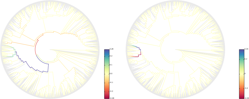
We here used the BV dataset of Srinivasan et al. [3] for testing, and refined the layout of the figures in Inkscape.

Furthermore, the projection of the eigenvectors can be used to get a scatter plot that shows how the samples are separated from each other by the PCA:

// Write out projection as a CSV file
auto const proj_fn = "path/to/projection.csv";
std::ofstream proj_os;
genesis::utils::file_output_stream( proj_fn, proj_os );
for( size_t r = 0; r < epca_data.projection.rows(); ++r ) {
    proj_os << sample_set.name_at(r);
    for( size_t c = 0; c < epca_data.projection.cols(); ++c ) {
        proj_os << "," << epca_data.projection( r, c );
    }
    proj_os << "\n";
}
proj_os.close();

This writes a simple CSV table file that can be opened with any spreadsheet program or read by Python or R for further analysis. We plotted the BV dataset as an example, colorized by the so-called Nugent score, which is a clinical indicator of the severeness of BV:

Edge PCA visualization of the projection as a scatter plot colorized by meta-data.

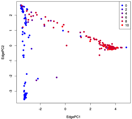
For details on the data, see Srinivasan et al. [3]. For more details on the implementation, see the gappa source code for Edge PCA.

Squash Clustering

Conducting Squash Clustering [1] is slightly more involved. We use an intermediate data structure to improve the speed and memory needs of the computations. This is for example used in the gappa implementation. Instead of storing the full placement data in a SampleSet as above, we only store the positions of the placement "masses" along the branches of the reference tree, and get rid of all the names of the pqueries, and other unnecessary detail such as pendant lengths. As Squash Clustering internally constructs additional trees for each inner cluster node, this saves memory. Furthermore, having the masses directly stored on the tree yields massive speedups (instead of having to iterate all pqueries to collect their masses).

The intermediate data structure is called MassTree, and is a specialization of the Tree data for edges and nodes as explained in the Data Model tutorial. Hence, we first first need to convert the SampleSet to this data structure:

std::vector<Tree> mass_trees;
for( auto const& sample : sample_set ) {
    mass_trees.push_back( convert_sample_to_mass_tree( sample, true ).first );
}

To actually save memory with this, we would need to free the sample_set afterwards (or even better, clear each Sample individually after conversion, as done in gappa, so that we do not need to keep everything in memory at the same time). However, for the sake of this tutorial, we keep the sample_set alive. We also need it later to get the names of the samples (which would need to be copied first, if one wants to clear the sample_set).

We can then set up an instance of the SquashClustering class, and run the analysis:

auto squash_clustering = SquashClustering();
squash_clustering.run( std::move( mass_trees ) );

The run function consumes the data (by moving it), again in order to save memory. If the MassTrees are needed later again, one has to store a copy, or recreate them. The instance then computes the cluster tree, which can be written to a newick file:

std::ofstream sc_tree_os;
file_output_stream( "path/to/cluster.newick", sc_tree_os );
sc_tree_os << squash_clustering.tree_string( sample_set.names() );
sc_tree_os.close();

Note that this tree is not a phylogenetic tree, but a cluster tree that shows which samples are clustered close to each other. See again Srinivasan et al. [3] for details. For the BV dataset, the tree looks like this:

Squash Cluster tree, with samples (tips) colorized by meta-data.

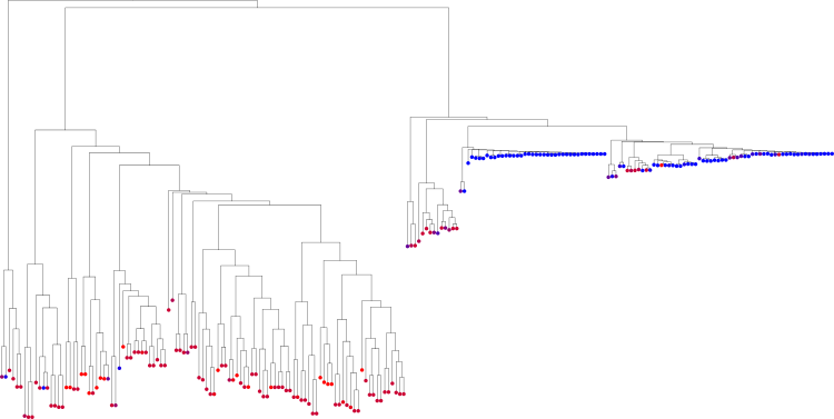
We here again used the Nugent score as explained above to colorize the tips of the tree, that is, the samples. This colorization was done as explained in the Tree Visualization tutorial.

Lastly, the SquashClustering class also supports functionals to set up progress reporting (it can take a while...), and to write out the mass trees of the inner cluster nodes, which represent all trees that are clustered below them in the hierarchical clustering.

Edge Dispersion and Edge Correlation

We introduced Edge Dispersion and Edge Correlation in [Czech et al., 2019] as two simple methods to visualize the reference tree based on differences between samples and their association with per-sample meta-data. In fact, the methods are simple enough that there is no separate function to compute them in genesis. Instead, we simple take the data, compute some numbers, and visualize them on the tree.

We here assume familiarity with the idea behind these methods. Both come in several flavors, in particular, both can be computed based on the placement masses per branch, or on the mass imbalances. Let's collect these data in two matrices:

// Get empty matrices of the correct size.
auto edge_masses     = Matrix<double>( sample_set.size(), tree.edge_count() );
auto edge_imbalances = Matrix<double>( sample_set.size(), tree.edge_count() );
 
// Fill them with the data.
for( size_t i = 0; i < sample_set.size(); ++i ) {
    auto const& sample = sample_set[i];
    edge_masses.row( i )     = placement_mass_per_edges_with_multiplicities( sample );
    edge_imbalances.row( i ) = epca_imbalance_vector( sample );
}

Now we can go ahead and compute the dispersions and correlations based on these matrices. For the dispersion, we first need the per-column means and standard deviations of the matrices. For simplicity, we here only continue considering the edge imbalances:

auto means_deviations = std::vector<MeanStddevPair>( edge_imbalances.cols(), { 0.0, 0.0 } );
for( size_t c = 0; c < edge_imbalances.cols(); ++c ) {
    means_deviations[c] = mean_stddev( edge_imbalances.col(c).begin(), edge_imbalances.col(c).end() );
}

From there, we can compute variance (squared standard deviation), the coefficient of variation (standard deviation divided by mean), and other measures, and visualize them on the tree as described in the Tree Visualization tutorial.

The Edge Correlation works similarly, with the addition of some meta-data feature being taken into account. For example, in case of the BV dataset, this could be the Nugent score, being read from a per-sample csv file using the CsvReader. Then, using either pearson_correlation_coefficient() or spearmans_rank_correlation_coefficient() on each of the matrix columns with the meta-data vector yields per-column (that is, per-edge) values that can again be visualized on the tree.

Phylogenetic k-means and Imbalance k-means

A different set of methods presented in [Czech et al., 2019] are two variants of the k-means method that can be used to cluster large numbers of samples. Phylogenetic k-means uses the KR distance between the samples to measure cluster similarity, while Imbalance k-means uses simple Euclidean distances on the imbalance vectors per sample.

Similar to Squash Clustering, we again use the MassTree data to simplify and speed up the calculations for Phylogenetic k-means. We here assume that the respective mass_trees data that we computed above in the Squash Clustering is still alive and was not destroyed there by moving it to the SquashClustering instance. Note that the KR distance for MassTrees is implemented in the earth_movers_distance() function.

For k-means, we need to set the number k of clusters to compute. Then, to run Phylogenetic k-means we do the computations using the MassTreeKmeans class:

size_t const k = 10;
auto phylogenetic_kmeans = MassTreeKmeans();
phylogenetic_kmeans.run( mass_trees, k );

The resulting clusters can then be accessed as follows:

auto const cluster_info = phylogenetic_kmeans.cluster_info( mass_trees );
auto const assignments = phylogenetic_kmeans.assignments();

This yields a KmeansClusteringInfo object that contains the variances of each cluster centroid, as well as the distances from each of the original data points to their assigned centroid. The second line yields the assignments of each data point (sample) to the clusters. That is, it is a vector of numbers 0 <= n < k that tells which sample was assigned to which of the k clusters.

The data can for example be accessed like this:

std::cout << "Sample\tCluster\tDistance\n";
for( size_t i = 0; i < assignments.size(); ++i ) {
    std::cout << sample_set.name_at(i);
    std::cout << "\t" << assignments[i];
    std::cout << "\t" << cluster_info.distances[i];
    std::cout << "\n";
}

The resulting table contains the number of the assigned cluster of each sample, as well as the distance between the cluster centroid and the sample.

The process for Imbalance k-means is similar. It uses EuclideanKmeans instead, using the imbalance data as input.

Placement-Factorization

Lastly, we briefly hint at a few details of how Placement-Factorization is implemented. See again [Czech et al., 2019] for the method description. To fully describe the implementation here would be too much for a simple tutorial. As however the involved methods are well documented, we here simply outline the workflow:

• The main method is phylogenetic_factorization(), which takes in the data that is needed to compute balances of samples, as well as an objective function used in the evaluation.
• To get that data needed for the balances, use the function mass_balance_data(), which can be configured via BalanceSettings, and returns a BalanceData object that is accepted by the phylogenetic_factorization() function.
• The result of running phylogenetic_factorization() is a vector of PhyloFactor objects for each of the factors that were identified by the algorithm. For each factor, one can obtain all information needed for further analysis and visualization, such as the index of the edge of the factor, the involved balances, and the values of the objective function.

The choice of objective function is depended on the user. In our implementation, we used a measure based on the fit of a Generalized Linear Model that describes how well the balances at an edge can be predicted from per-sample meta-data:

auto objective_function = [&]( std::vector<double> const& balances ){
    auto const fit = glm_fit( meta_data, balances, glm_family_gaussian() );
    return fit.null_deviance - fit.deviance;
}

This function can simply be plugged into the phylogenetic_factorization(). For details on the choice of objective function, see the excellent paper by [Washburne et al., 2017].

References

[1] F. Matsen, S. Evans, Edge Principal Components and Squash Clustering: Using the Special Structure of Phylogenetic Placement Data for Sample Comparison, PLoS One, vol. 8, no. 3, pp. 1-15, 2013. DOI: 10.1371/journal.pone.0056859

[2] L. Czech, A. Stamatakis, Scalable methods for analyzing and visualizing phylogenetic placement of metagenomic samples, PLOS ONE, vol. 14, no. 5, pp. e0217050, 2019. DOI: 10.1371/journal.pone.0217050

[3] S. Srinivasan, N. Hoffman, M. Morgan, F. Matsen, T. Fiedler, R. Hall, D. Fredricks, Bacterial communities in women with bacterial vaginosis: High resolution phylogenetic analyses reveal relationships of microbiota to clinical criteria, PLOS ONE, vol. 7, no. 6, pp. e37818, 2012. DOI: 10.1371/journal.pone.0037818

[4] F. A. Matsen, N. G. Hoffman, A. Gallagher, and A. Stamatakis, A format for phylogenetic placements, PLoS One, vol. 7, no. 2, pp. 1–4, Jan. 2012. DOI: 10.1371/journal.pone.0031009

[5] A. D. Washburne, J. D. Silverman, J. W. Leff, D. J. Bennett, J. L. Darcy, S. Mukherjee, N. Fierer, and L. A. David, Phylogenetic factorization of compositional data yields lineage-level associations in microbiome datasets, PeerJ, vol. 5, p. e2969, Feb. 2017. DOI: 10.7717/peerj.2969