Tree Structure Revisited

The introduction in Tree Basics gave an overview of how to do some basic tasks with trees. For most needs however, a deeper understanding of the underlying data structure is needed, which we provide here.

As stated before, the elements of a Tree are:

The Nodes and Edges are an abstraction on top of the tree topology that is used to store data and to give unique identifiers in algorithms. However, the topology itself is defined via Links - they connect Nodes and Edges with each other and link to neighbouring Links. Each Edge has two Links associated with it, and each Node has as many Links associated as it has Edges (and hence, neighbouring Nodes) next to it.

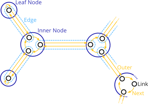
Tree structure with Links, Nodes and Edges.

The yellow arrows in the figure are the connections between Links that define the topology. Each Link has a next() Link, which is its neighbour within the same Node, as well as an outer() Link, which is its counterpart in the Node along the Edge that is associated with the Link. Hence, one can traverse the tree by following the Links:

next().outer().next().outer() ...

This yields an Eulertour of the tree, and is in fact how the iterators and traversals presented before work. Given a Link, by following all next() links until one reaches the given Link again, one can count the number of edges (degree) of the Node associated with the Link. In particular, Links that belong to leaf nodes of the tree have a next() link that points to themselves.

Switching between Links, Nodes and Edges

The Tree data structure hence uses Links to define the tree topology: The next() and outer() links allow to traverse the tree. The Nodes and Edges of the Tree on the other hand do not contain any topological information; they are meant to provide an abstraction on top of the topology that is more useful in algorithms.

One can switch from a Link to its associated Edge and Node via the edge() and node() functions. To get from a Node to one of its Links, use primary_link(), which will give the Link that is in the direction towards the root. For Edges, we also distinguish between the directions towards and away from the root; they offer functions primary_link() and secondary_link(), respectively.

By having the direction towards the root captured in the tree topology this way, algorithms can leverage this information. For example, to quickly find the path towards to root from a given node, one can use:

node --> primary link --> outer link --> node --> primary link --> ...

Of course, the root of the tree can also be directly accessed via root_node(). Note that trees in genesis are internally always rooted in the sense that there is such a node towards all primary links lead. However, whether the tree is rooted in the biological sense simply depends on whether the root node has two or more neighbors. See below for details.

Indices of Links, Nodes, and Edges

Each Link, Node, and Edge contains an index() property. For each of the three, the indices are consecutive zero-based numbers, that are stable for a given Tree. Two trees that are read from the same Newick file for example will have the same indices for their Links, Nodes, and Edges. Indices of given elements only change if parts of the tree are deleted. Note however that the order of indices is arbitrary and does not necessarily follow any traversal order.

These indices hence can be used to refer to elements of the Tree, for example via Tree::node_at(), instead of storing pointers to them. Furthermore, they are extensively used in genesis as indices in vectors and matrices. For example, a pairwise distance matrix between nodes in a Tree can use their indices as indices in the matrix, as done in node_branch_length_distance_matrix().

The Tree also has accessors such as Tree::links(), Tree::nodes(), and Tree::edges(), that allow to iterate all the elements in their index order. This is the fastest way of iteration, and particularly useful to fill index-based vectors and matrices:

// Prepare a vector of all node names.
auto names = std::vector<std::string>( tree.node_count() );
 
// Traverse the Nodes of a Tree, and fill the vector.
for( auto const& node : tree.nodes() ) {
    names[ node.index() ] = node.data<CommonNodeData>().name;
}

The Nodes and Edges of the Tree are also able to store arbitrary extra data, as explained below in Data Model.

Rooting and Types of Nodes

As mentioned above, trees in genesis are always rooted in the sense that there is one "starting" node from which tree traversals begin (unless a specific node to start from is provided). However, they are not necessarily rooted in the biological sense.

Tree rooting.

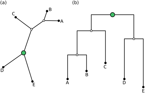
The tree in (a) above is unrooted in the biologocal sense, and drawn that way. However, the green node serves as a so-called top-level trifurcation, that is, it is the root node for the tree structure in genesis. On the other hand, the tree in (b) is rooted on an edge, and hence has a top-level bifurcation that serves as the root.

In genesis, both trees are treated completely the same - they are not identical, as (b) has one additional node (its green root node), but they both just use the normal Tree datastructure. A rooted and an unrooted tree can be distinguished by the number of neighbouring nodes of the root: in (a), there are three neighbours, in (b) there are only two. This is for example how the is_rooted() function works.

Apart from that distinction, all nodes in a tree are treated the same. The only ways in which the root information is stored in the tree is via the root_link() of the tree, as well as the implicit information provided via the primary links of the nodes in the tree.

Data Model

So far, we have seen the use of Node and Edge data in the form of

node.data<CommonNodeData>().name;
edge.data<CommonEdgeData>().branch_length;

Each Node and each Edge has such a data<>() function, that needs a template parameter to know which particular type of data is associated with the node or edge. The nodes and edges can hold any data<> that is derived from BaseNodeData and BaseEdgeData, respectively.

The most common example of such data classes are CommonNodeData and CommonEdgeData, which provide the defaults for most standard use cases. They provide taxon names, and branch lenghts, as shown in the code snipped above. Both serve as an example of how to correctly derive from the base classes (which do not hold any data) in order to create custom data classes for the nodes and edges.

Reading and Writing Revisited

In the Tree Basics Reading and Writing section, we have seen how to read a tree from a Newick file:

// Read a Newick file into a Tree object.

Tree tree = CommonTreeNewickReader().read( from_file( "path/to/tree.newick" ));

With the above Data Model section, we can now better understand how the tree reading works: The instance of CommonTreeNewickReader that is used in the code snipped is a specialization of the general NewickReader class, which is able to parse newick files. The specialization then adds a layer on top that understands the taxa names and the branch lengths that are present in a typical newick tree, creates a tree with CommonNodeData and CommonEdgeData data types at the nodes and edges, and fills them with the respective data found in the input newick tree.

We use this abstraction of "basic tree reader" plus "special layer for the actual data" in order to allow for trees that accommodate different types of data and meta-data. In particular, the newick file format only specifies taxon names and branch lengths in the standard. However, often there is additional data such as bootstrap support values, or edge numbers as used in phylogenetic placement, that are not part of newick itself. Instead, these extensions "misuse" features such as comments (denoted as square brackets [] in newick strings) to store such additional data. Hence, the semantics of such data is not clear if one is given a newick tree without further information.

For example, the tree

((C,D)[&!color=#009966],(A,(B,X)[&bs=82,!color=#009966])[&bs=70],E);

contains some information about color and bs (bootstrap support) that are non-standard. Consequently, our reader allows to customize how such data is interpreted and stored in the resulting Tree object.

Note that by default, the Tree does not support color or bootstrap support values - if needed, these could be implemented as new node and edge data types, as explained in the Data Model section. Then, in order to store data at the respective nodes and edges when reading a tree, the NewickReader has several plugin points for functions that are called whenever data for nodes and edges is parsed while reading the tree. See CommonTreeNewickReaderPlugin for examples of how this can be implemented.

This technique works the same for writing trees. There, the plugin functions for NewickWriter and PhyloxmlWriter allow to customize how data that is stored in a Tree object is turned into strings to be stored in the output files.

Remark: See Czech et al. 2017 for a comprehensive review on the issue of tree data storage in the Newick file format.

Tree Manipulation

We also provide some simple tree manipulation methods for basic tasks. Complex tree moves (SPR, TBR, NNI, or similar topological rearrangement methods) are currently not implemented.

High Level

A good starting point to explore tree manipulation is minimal_tree_topology(), which returns a minimal tree with two nodes, connected by an edge. The function sets up the basic objects, including the respective links, and connects them to each other. A similar function is minimal_tree(), which additionally sets the data of the nodes and edges.

Given a Tree, one can then use functions such as add_new_node() (in multiple variants) and delete_node() and its variants for basic high-level tree manipulation. Functions for rooting (make_rooted()), unrooting (make_unrooted()) and rerooting (change_rooting()) are also provided.

Low Level

All the above functions internally use (quite extensive) manipulation of the pointers in the Nodes, Edges, and Links to achieve the desired effects. In other words, they reset where next() and outer() Links point to, etc. This looks quite involved at first glance, but using the exemplary figure above, one can track the changes and write their own tree manipulation functions as needed. The exemplary high-level functions listed above should suffice as code examples to get started.