Phylogenetic Trees

Phylogenetic trees, or phylogenies, are a representation of the evolutionary history of species. The leaf nodes usually represent extant species (which have a species name assigned), while the inner nodes are their putative ancestors (usually without a name). The edges that connect those nodes often have a branch length assigned, which indicates the "amount of evolution" that happened between the two nodes at the ends of the edge.

The trees can be either rooted or unrooted. In a rooted tree, there is a top level root node, which symbolizes the "origin" of the tree, that is, the common ancestor of all other nodes in the tree. As the "origin" of evolution might not be clear in some cases, there are also unrooted trees, which do not have a top level root node.

Tree Structure

Phylogenetic trees can be quite complex: they can have different types of topologies (rooted/unrooted, bifurctating/multifurcating), there are different operations we want to do (e.g., preorder and postorder traversal), and we also want to store arbitrary data on the nodes and edges. Thus, there is a lot to explain.

Rooted vs Unrooted Trees

In Genesis, both rooted and unrooted phylogenies are modeled in the Tree data structure, which represents an inherently unrooted tree. This data structure makes it possible to inspect the tree from any given node in the same manner - that is, without the need to distinguish between parent and child nodes. It also allows for multifurcations, i.e., Trees in Genesis don't have to be binary/bifurctating.

The notation of a root node is however still important in many cases, for example when Traversing the Tree, because the traversal has to start somewhere. To this end, there is always one special node marked as "root" of the tree - which is usually set to be the root of e.g., the Newick input tree. Note that, this root node is also present in unrooted trees - in this case, we can call it a "virtual" root node.

In other words: Trees in Genesis are stored in an unrooted way (no parent-and-child structure), yet we always mark a special node as root, which is used as a "hook" for starting traversals and other operations. Other than that, the root node is just a normal Node of the Tree.

When working with Trees from input files like Newick, this comes in handy: File formats often store the tree structure starting from a root. This information is kept when reading the file in Genesis via the root node marker. However, we are still free to traverse the Tree as if it was unrooted. When writing a Tree back to a file, this root marker is again used as the actual root in the file format.

Elements of a Tree

The main elements of a Tree in Genesis are:

The purpose of Links is explained later in Tree Structure Revisited; for now, we will focus on Nodes and Edges:

Nodes and Edges of an unrooted multifurcating Tree.

Genesis allows to store arbitrary data on the Nodes and Edges of a Tree. For many use cases, there are two important variables:

Node names
Branch lengths

For this simple, typical use case, we offer the CommonTree. It is an alias for a Tree that stores a name string at each Node and a branch_length at each Edge. For more information about storing data on Trees, see Data Model.

Now, it's time to dive into some code!

The examples in this tutorial assume that you use

#include "genesis/genesis.hpp"
using namespace genesis::tree;
using namespace genesis::utils;

at the beginning of your code.

Reading and Writing

Reading from a Newick file with node names and branch lengths is achieved via a CommonTreeNewickReader:

// Read a Newick file into a Tree object.

Tree tree = CommonTreeNewickReader().read( from_file( "path/to/tree.newick" ));

It is also possible to read trees stored in strings. For example, the tree from above can be stored in Newick like this

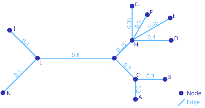
(((A:0.2,B:0.3)C:0.3,(D:0.4,E:0.45,F:0.3,G:0.35)H:0.25)I:0.8,J:0.4,K:0.5)L;

which uses node "L" as the (virtual) root. Reading is then:

// Given a string containing a Newick tree, read it into a Tree object.
std::string newick = "(((A:0.2,B:0.3)C:0.3,(D:0.4,E:0.45,F:0.3,G:0.35)H:0.25)I:0.8,J:0.4,K:0.5)L;";
tree = CommonTreeNewickReader().read( from_string( newick ));

Writing a Tree to Newick and PhyloXML works similarly, using CommonTreeNewickWriter and CommonTreePhyloxmlWriter:

// Write a Tree to a Newick file and a PhyloXML file.
CommonTreeNewickWriter().write( tree, to_file( "path/to/tree.nw" ));
CommonTreePhyloxmlWriter().write( tree, to_file( "path/to/tree.phyloxml" ));

For more details, particularly on how to read different data for the nodes and edges, see Reading and Writing Revisited.

Inspecting a Tree

Printing a simple overview of the topology for Tress can be done using PrinterCompact:

// Print the tree topology including node names and branch lengths.

std::cout << PrinterCompact().print( tree );

For the tree from above, this yields

L: 0.8
├── I: 0.8
│   ├── C: 0.3
│   │   ├── A: 0.2
│   │   └── B: 0.3
│   └── H: 0.25
│       ├── D: 0.4
│       ├── E: 0.45
│       ├── F: 0.3
│       └── G: 0.35
├── J: 0.4
└── K: 0.5

It can also be customized to other than the default data types. Furthermore, for inspecting the Tree data structure in more detail, we offer PrinterDetailed and PrinterTable. All of this however assumes that you first read the Tree Advanced tutorial.

Iterating Nodes and Edges

It is often necessary to get information about Nodes and Edges of a Tree, without actual need to use the Tree topology, for example to simply print all node names or branch lengths:

// Print all node names.
for( auto const& node : tree.nodes() ) {
    auto const& name = node.data<CommonNodeData>().name;
    if( ! name.empty() ) {
        std::cout << name << std::endl;
    }
}
 
// Print all branch lenghts.
for( auto const& edge : tree.edges() ) {
    auto const& branch_length = edge.data<CommonEdgeData>().branch_length;
    std::cout << branch_length << std::endl;
}

The above code gets the data of Nodes and Edges via the data<>() cast function. Details of this are later explained in Data Model.

In addition to this, it is also possible to access the Tree elements via their index. This is useful for creating and storing additional information, for example by using the same indices to refer to elements in a std::vector or a Matrix:

// Iterate nodes using their index and fill a vector with them.
auto names = std::vector<std::string>( tree.node_count(), "" );
for( size_t i = 0; i < tree.node_count(); ++i ) {
    auto const& node = tree.node_at( i );
    auto const& name = node.data<CommonNodeData>().name;
    names[ i ] = name;
}
 
// Iterate edges using their index and fill a vector with them.
auto branch_lengths =  std::vector<double>( tree.edge_count(), 0.0 );
for( size_t i = 0; i < tree.edge_count(); ++i ) {
    auto const& edge = tree.edge_at( i );
    auto const& branch_length = edge.data<CommonEdgeData>().branch_length;
    branch_lengths[ i ] = branch_length;
}

The code above is a bit wasteful by first default-constructing the vector elements and then assigning to them again - this is for illustration purposes only.

Lastly, the same also works for Links, see Tree Structure Revisited for details on them.

Note that, all the above examples iterate the Nodes and Edges in the order in which they are stored in the Tree object - this order is independent of any traversal order. See the next chapter Traversing the Tree for ways to do traversals along the Nodes and Edges of a Tree.

Traversing the Tree

Traversing a Tree in a specific order can easily be done using the Tree traversal iterators.

Eulertour Traversal

All Tree traversal iterators are based on a round trip around the Nodes and Edges of the Tree. This is due to the way the Tree is structured internally, see Tree Structure Revisited for details. Such a round trip is also called an Euler tour of the Tree, see Euler tour technique for an explanation. It looks like this:

Eulertour Traversal of a Tree.

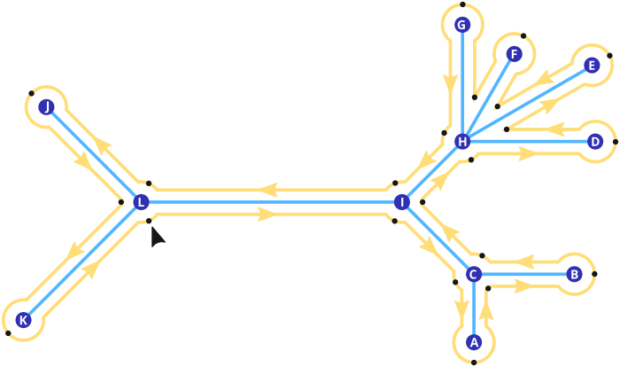
The yellow line indicates the course of the Eulertour, while the yellow arrows on it indicate the direction. Black dots along the line mark nodes that are visited during the traversal. The black arrow at node "L" indicates the start of the tour, as this is marked as the root node of the Tree.

We can output the Nodes which are visited during the Euler tour like this:

// Do an eulertour around the Tree and print Node names.
for( auto it : eulertour( tree ) ) {
    std::cout << it.node().data<CommonNodeData>().name << " ";
}
std::cout << std::endl;

The above traversal prints

L I C A C B C I H D H E H F H G H I L J L K

It is also possible to start at a different Node:

// Find Node "C" and start an Eulertour traversal from there.
auto node_C = find_node( tree, "C" );
for( auto it : eulertour( *node_C ) ) {
    std::cout << it.node().data<CommonNodeData>().name << " ";
}
std::cout << std::endl;

This prints

C I H D H E H F H G H I L J L K L I C A C B

As one can see, the traversal first moves into the direction of the root Node "L". This can be changed using Links, see Tree Structure Revisited for details on them.

Preorder and Postorder Traversal

Using the Tree from above, we can iterate its Nodes in preorder fashion like this:

// Traverse the Tree in preorder fashion, starting from the root Node "L".
for( auto it : preorder( tree ) ) {
    std::cout << it.node().data<CommonNodeData>().name << " ";
}
std::cout << std::endl;

This yields

L I C A B H D E F G J K

Similarly, to do a postorder traversal, we can use:

// Traverse the Tree in postorder fashion, starting from the root Node "L".
for( auto it : postorder( tree ) ) {
    std::cout << it.node().data<CommonNodeData>().name << " ";
}
std::cout << std::endl;

This prints

A B C D E F G H I J K L

Remark: It is not a coincidence that this is in alphabetical order. If you again inspect the Newick tree that was read to get this tree, you will notice that its nodes are also stored in alphabetical order. This means that Newick internally stores the nodes in postorder fashion.

We can also start the traversals from any other Node (or any other direction, using Links), in the same way as shown for the Eulertour traversal:

// Find Node "H" and start traversals from there.
auto node_H = find_node( tree, "H" );
for( auto it : preorder( *node_H ) ) {
    // ...
}
for( auto it : postorder( *node_H ) ) {
    // ...
}

It is important to note that the preorder and postorder traversal iterators do a node-based traversal of the Tree. That means, each Node is visited exactly once. The iterators however are also useful to traverse Edges of the Tree.

When using such node-based traversals to iterate over the edges of the tree, exactly one Edge is visited twice - this is always one of the Edges that belong to the starting node of the traversal (i.e., in the examples above, either the root, or node "H"). In a preorder traversal, the first stop of the iterator is at the start node; for postorder traversal, the last stop is at the start node. Thus, in order to not process an Edge of this node twice, the iterators offer those functions:

Preorder Iterator: is_first_iteration()
Postorder Iterator: is_last_iteration()

They are used like this:

// Do a preorder traversal of the Edges, and print their branch lengths.
for( auto it : preorder( tree ) ) {
    if( ! it.is_first_iteration() ) {
        std::cout << it.edge().data<CommonEdgeData>().branch_length << " ";
    }
}
std::cout << std::endl;
 
// Do a postorder traversal of the Edges, and print their branch lengths.
for( auto it : postorder( tree ) ) {
    if( ! it.is_last_iteration() ) {
        std::cout << it.edge().data<CommonEdgeData>().branch_length << " ";
    }
}
std::cout << std::endl;

This prints

0.8 0.3 0.2 0.3 0.25 0.4 0.45 0.3 0.35 0.4 0.5
0.2 0.3 0.3 0.4 0.45 0.3 0.35 0.25 0.8 0.4 0.5

We see that each branch length appears exactly once.

Levelorder Traversal

In some cases, one needs to compute values starting from inner nodes outward, for instance, for pairwise distances between nodes (as implemented in node_branch_length_distance_matrix()). While a preorder traversal does work for this, a level order traversal might conceptually be simpler:

Levelorder Traversal of a Tree.

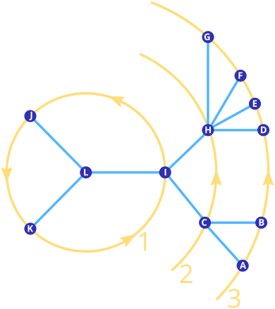
The traversal starts at the root node (or, if provided, an arbitrary other node), and then spirals outward. Within each level, the order is the same in which the subset of nodes would be visited in an Eulertour traversal.

The iterator is used like this:

// Traverse the Tree in levelorder fashion, starting from the root Node "L".
for( auto it : levelorder( tree ) ) {
    std::cout << it.node().data<CommonNodeData>().name << " ";
}
std::cout << std::endl;

This prints

L I J K C H A B D E F G

As before, the iterator offers a function is_first_iteration() that can be used to skip the stop at the starting node, which is useful when iterating edges instead of nodes. Furthermore, the depth() function can be used to get the level (depth with respect to the starting node) of the current node. Note also that the iterator again can take an arbitrary node as starting node instead of using the root, by calling it via levelorder( node ).

Path Traversal

For some special algorithms, one might want to traverse the path between specific nodes. To this end, we offer an iterator that works like this:

// Traverse a path between two nodes in the tree.
auto node_A = find_node( tree, "A" );
auto node_D = find_node( tree, "D" );
for( auto it : path( *node_A, *node_D ) ) {
    std::cout << it.node().data<CommonNodeData>().name << " ";
}
std::cout << std::endl;

This prints

A C I H D

Instead of the first/last iteration functions offered by the other iterators, this one has a function is_last_common_ancestor() that serves the same purpose. This is because the path between two nodes always contains their last common ancestor, which is the node whose adjacent edges are both visited by the iterator.

Furthermore, this function is useful when the LCA of the two nodes is needed for the algorithm. However, using this method to find LCAs is inefficient. See the LcaLookup class for a better approach to finding LCAs of nodes. Also, for individual LCAs, one can use lowest_common_ancestor() or lowest_common_ancestors() to get a full matrix of LCAs.

We also offer a path_set() iterator, which is slightly more efficient, and hence meant for speed-sensitive applications, but visits the nodes in a different order.