Visualize Placements

Summary

Takes one or more jplace file(s) and visualizes the distribution of Pqueries on the reference tree (that is, the number of placements per branch). For this, it uses color coding and outputs a Nexus file.

This demo is located at

genesis/doc/code/demos/visualize_placements.cpp

Details

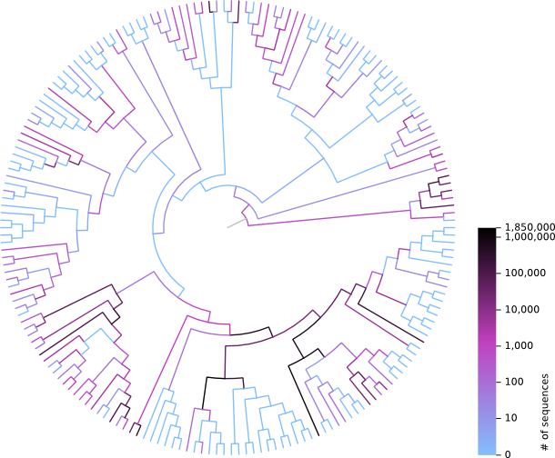
The program takes a path to either a jplace file, or a directory containing jplace files, reads all of them and counts the placement mass (according to the like_weight_ratio of each placement) for each branch of the tree. Those masses are then turned into colors representing a heat gradient of how much placement mass was placed on each branch, and writes a tree with this color information to a given nexus file path. The resulting file can be read and visualized with, e.g., FigTree:

Tree with branches colored according to weight of placements on the branches.

If a directory is given as first command line argument, all files in it that end in ".jplace" are processed and their weights are accumulated. This means that all trees in the jplace files need to have the same topology. For reasons of simplicity, we only check if they have the correct number of edges. It is thus up to the user to make sure that all trees have identical topology. Otherwise, the result will be meaningless. If for example EPA was run multiple times with different sets of query sequences, but always the same reference tree, the resulting jplace files can be used here.

If a single file is given as input, all of the above is obsolete. The filename also does not need to end in ".jplace" in this case. In this case, simply this file is visualized.

Furthermore, as second command line argument, the user needs to provide a valid filename for the output nexus file. That means, the path to the file needs to exist, but the file not (yet).

The program prints output that shows the used color gradient and furthermore lists the positions on this gradient that correspond to certain placement masses. Particularly, as we use a log scale for coloring, the printed positions are multiples of ten, and finally the maximum mass, which always corresponds to the end of the color gradient, i.e., black color.